\(χ^2\) test
What if you don't have data that can be summarised in the usual ways?
Most statistical tests deal with data in the form of scores which can be represented with a frequency distribution. This is known as continuous data, and one of its characteristics is that it makes sense to calculate the mean, standard deviation, etc.
Some data however is not continuous - it is divided into categories where it makes no sense to calculate the usual statistics. If you were to ask people, for example, to tell you their preferred social networking site and responses were split between Facebook and Twitter, it makes no sense to try to calculate the mean of these two responses. This kind of data is categorical data, and requires a different kind of test.
Background
The test discussed here is known by the Greek letter \(χ\) (chi - pronounced 'kai'). The full name of chi square comes from the way the result is calculated as you will see below.
\(χ^2\) can be used in two different ways. The first is to test for a significant difference between two categories as in the social networking example above. This is known as a goodness-of-fit test, because it compares how well the observed data fits the expected data.
The second is to test whether there is a significant association between two categorical variables. This second use is similar to the use of Pearson's r in testing the correlation between two continuous variables, and is known as a test of independence.
The central insight is that in random data, there will be a roughly equal number of observations in different categories. For example, when a fair coin is flipped 100 times, it will come down heads around 50 times. There will some natural variation, but we can say that the expected frequency is the number of trials, N, divided by the number of categories, k. The \(χ^2\) test basically compares the actual number of observations to the expected number.
Assumptions
As with other tests, there are some assumptions that should be checked to ensure that the results of a \(χ^2\) test is valid.
- All observations are independent of each other
- The dataset is of adequate size
- Each category is adequately represented
The 'adequacy' referred to in the assumptions is not absoultely fixed, although there are established conventions. As a minimum, there must be more observations than categories; however, larger samples will give more reliable results. With small datasets, there is the possibility of a Type II error.
The third assumption is a better validity criterion from a practical point of view. Although practice differs, you should ensure that there is a minimum of five observations expected in any single category. That way, the overall size of the dataset will be guaranteed to exceed the number of categories.
From a practical point of view, it can be useful to combine some of the lower-frequency categories into a single one called "Others".
Practical exercise: \(χ^2\) for goodness-of-fit
In this exercise, we will be using the results from a small survey of students who were asked for their preferred social media service along with some other data. We will be using the data to determine whether the preference for Facebook is statistically significant.
In a real situation, we would expect the dataset to be a lot larger than the example we are using here.
Excel does not provide a single function to do the whole job in this case, but it does provide a function that calculates the probability associated with a particular value of the \(χ^2\) statistic.
The Excel functions shown in the image below go through the mathematical steps required to calculate \(χ^2\) and then determine its probability using the built-in function. To simplify the calculation, the less popular sites have been combined into a single category labelled Others.
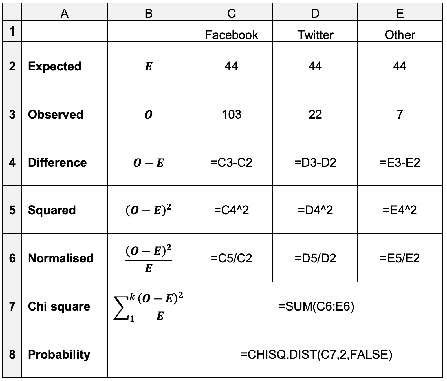
Table 1: \(χ^2\) for goodness-of-fit
The values in row 2 are equal: they represent the theoretical count of values under the null hypothesis. This is calculated by dividing the number of observations by the number of categories.
You can use the Excel COUNTIF function to help calculate the values in row 3.
The remaining formulae are shown in the image. The final mathematical representation in row 7 is the formula for \(χ^2\).
The second parameter to the CHISQ.DIST function is the degrees of freedom, df. Remember that df
is often related to the number of subjects or groups minus one. Here, it is one less than the
number of categories.
If the preference for Facebook is significant at the 95% level, the calculated probability will be less than 0.05.
Practical exercise: \(χ^2\) for independence
In this exercise, you will answer the question, "Is preferred social networking site related to gender?".
Both of the variables we are interested in are categorical: gender is either female or male, and site preference is the name of a particular site. So in this case there are two variables, whereas in the previous exercise there was only one. The \(χ^2\) test is therefore slightly different. Each variable has two levels, so this test is described as a 2x2 \(χ^2\) test.
Starting with the social media survey data in its original format, remove all columns except gender and site preference, and delete any rows where no preference is stated. There are only a few instances of the less popular sites, so we will also remove those rows leaving only Facebook and Twitter.
The \(χ^2\) statistic is calculated in a similar as it was in the previous exercise by squaring the difference between the expected and observed values. The expected values are calculated based on the assumption that the preferences of one category are the sameas the preferences in the whole population. That is, if there is no gender bias, the proportion of male students who prefer Twitter will be equal to the proportion of female students who prefer Twitter, and that will also be equal to the preference in the overall population. The expected values can be calculated by setting out the table shown below in Excel.
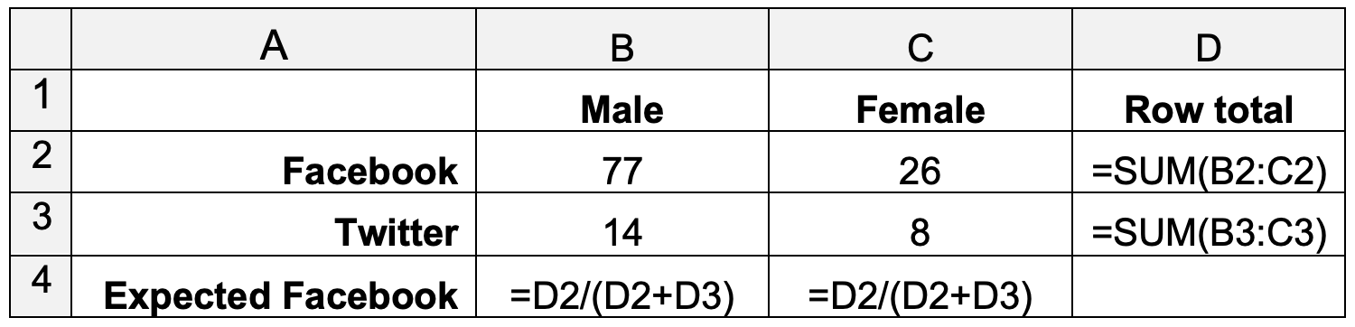
Table 2: Expected values
The number of occurrences can be counted by using the Excel COUNTIFS function.
To calculate \(χ^2\), set out a second table as shown below.
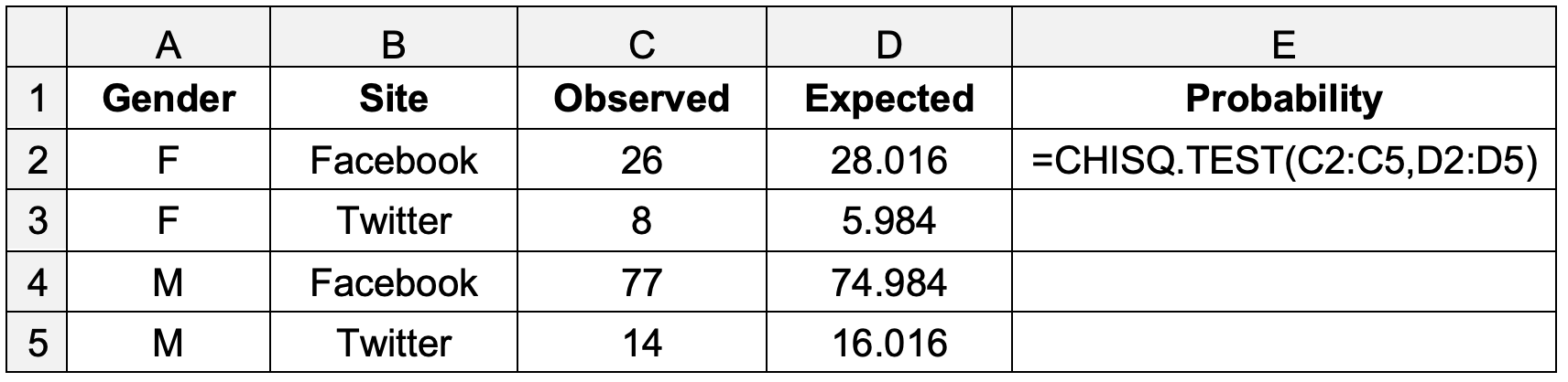
Table 3: \(χ^2\) for independence
The value in row 4 of table 2 represents the expected proportion of Facebook preferences, \(fb\%\). The expected number of Facebook preferences for female students is just \(fb\%\) multiplied by the total number of female students. The expected number of Twitter preferences is calculated as \(1-fb\%\) multiplied by the total number of female students.
If the observed difference in site preference between male and female students is significant at the 95% level, the probability calculated in cell E2 in Table 3 will be less than 0.05.
