PID controller theory
There is a large body of theory relating to the behaviour of general systems which requires some complex mathematics. Fortunately, there are some more pragmatic approaches that have been proven to be effective in a wide range of situations. This section will explore one of the most common types of controller for which there is support in a wide range of development environments including Arduino. We need to set the problem up first though in order to understand the solution.
Consider the problem of maintaining the correct proportion of a chemical in an industrial process. As the chemical gets used up, it needs to be replaced. Just maintaining a constant flow is not an effective strategy because of other variable quantities in the system. The only way to know how much chemical to add at a given moment is to measure the actual concentration with a sensor. This is one particular example of a feedback loop. All precision control scenarios involve feedback loops on one sort or another. The diagram in Figure 2 represents the general case in the form of a block diagram.
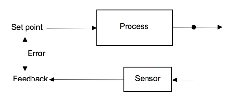 Figure 1: A simple feedback loop
The set point is the required value - in our example this is the concentration of a chemical, but it could be any quantity of interest such as speed, temperature, direction, etc. The difference between the set point and the measured value represents the error that needs to be corrected. The next question is how to use the feedback to correct the behaviour of the system. First we will introduce the idea of a controller which takes the error as an input and sends a modified control instruction into the process instead of just the set point. This is illustrated in Figure 2.
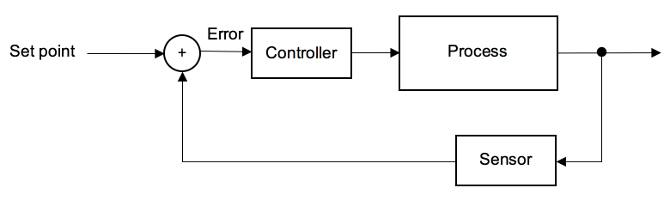 Figure 2: System block diagram showing the controller
The circular element labelled with a plus sign performs an addition or subtraction on its inputs, which in this case are the set point and the measured error. The symbol for this element can take several possible forms. Sometimes it is shown with an explicit minus sign, and sometimes it is shown with a capital sigma (Σ) to represent a mathematical sum. They are all equivalent, and some familiarity with block diagrams is assumed when interpreting a block diagram.
Proportional control
The question now is what the controller does with the error value. One possibility would be to make an adjustment to the input signal that is proportional to the error - ie multiply the error by some factor and add the result to the signal. This would capture some of the behaviour of the steam governor: a larger error would produce a larger responses, and hence a stronger correction. There is a dilemma here though because the correction replies on the existence of an error. Once the desired process value is achieved, the error would drop to zero and consequently, so would the correction. Any systematic drift in the process would then reoccur and the process value would start to deviate again. Depending on the speed at which the controller applies the correction, the result might appear as an oscillation in the process variable, or as a small persistent offset from the desired value.
Proportional-Integral control
A solution to the problem with instantaneous reliance on the error value would be to keep track of past errors. That way, even if the error value does drop to zero, we have a memory of the appropriate correction to apply. In mathematical terms a running accumulation of past values is an integral. Adding a proportional correction and an integral correction to the process signal can therefore eliminate the offset problem.
Control actions are often studies in relation to a step change in the set point. The graph of the desired change might look like the blue trace in Figure 3: the set point starts low and suddenly jumps up to a higher level. The job of the controller is to guide the system from the first operational context to the second. Because a step change in the set point appears to the controller as a large error, it makes relative large adjustments to the input signal. This can lead to an overshoot in the behaviour of the system as shown by the red trace in Figure 4. Once the process value exceeds the set point, the sign of the error changes and the value of the integral correction starts to shrink. A little later (around 5s in Figure 4), the process value drops below the set point, and the error sign changes again so that the integral term starts to grow again. This behaviour continues until the process has settled around the new set point.
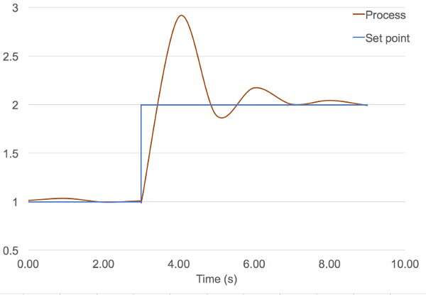 Figure 3: Behaviour of a PI controller
Clearly, the large overshoot just after the set point changes is not desirable. Depending on the type of process being controlled, such a large deviation from the expected value could cause damage to equipment or product. A further step is therefore necessary to remove this problem.
Proportional-Integral-Derivative (PID) control
The third and final step is to take into account the rate of change of the error term. When the error is increasing, the correction needs to be large in order to compensate. When the error is decreasing, however, the process value is approaching the set point and so we need to reduce the error term accordingly. Once the error reaches zero, we want the correction term to be equal only to any systematic offset. In mathematical terms, the rate of change of a variable is a derivative, and adding an appropriate derivative term can damp the system response so that overshoot is eliminated. The behaviour of the PID controller is illustrated in Figure 4. The system still takes a short time to settle at its new value but it is roughly the same as for the PI controller. The big difference is that the overshoot is completely eliminated.
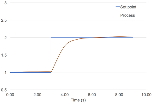 Figure 4: Behaviour of a PID controller
The correction terms that have been applied to create the charts in Figures 3 and 4 are also multiplied by coefficients to produce optimal behaviour. The appropriate coefficients to use in a given situation can be found in a number of ways including trial-and-error. The process of identifying appropriate coefficients is know as tuning the controller.
The maths
The full equation for a PID controller appears quite complex:
In the equation, the left-hand side represents the value of the controller output, \(u\), at time \(t\). On the right-hand side, there are three terms separated by plus signs. The first is the proportional term where the error at time \(t\), \(e(t)\), is simply multiplied by the proportional coefficient, \(K_p\). The second term is the integral term multiplied by the integral coefficient, \(K_i\), and the third follows the same pattern being the derivative term multiplied by the derivative coefficient, \(K_d\).
The equation can be presented more simply as
where \(P\), \(I\) and \(D\) represent the proportional, integral and derivative terms, and \(K_p\), \(K_i\) and \(K_p\) are the coefficients as before.