Preprocessing
Digitised signals in their raw form may contain errors or gaps, and may contain more detail than is actually useful. Before performing any processing, it is sometimes useful to perform preprocessing in order to clean the data.
Outliers
Some sensors, such as the sensitive instruments used to measure gas exchange, can produce erroneous large values in response to electromagnetic disturbances or other external influences. These spurious values, known as spikes or outliers can bias the overall signal and have a damaging effect on any later processing. The typical solution is to remove them; however, this raises the question of how big a spike needs to be before it is removed. Although the answer may vary from one application to another, a typical rule is to classify any value which deviates from the mean by more than three standard deviations as a spike. This is illustrated in Figure 4 where the mean is represented by the green dashed line and the orange dashed line corresponds to the mean plus three times the standard deviation. There is one obvious spike which should be removed. If it is important to keep the row so that no timesteps are lost, the spike value could be replaced with the mean of the preceding and following values.

Figure 4: Outlier
Gaps
Gaps may appear in time series data for many reasons including sensor faults. Various strategies can be employed for dealing with them, the simplest being to forward fill or backward fill. In a forward-fill strategy, the previous measured value is used to fill the gap, and in a backward-fill strategy, the next valid measured value is used. Forward filling is easy to implement in a microprocessor sketch, and represents a simple choice of approach.
For more accuracy, an interpolation approach can be employed. With this strategy, the missing values are calculated based on the last valid value before the gap and the first valid value following the gap. Different mathematical functions can be used, but the simplest choice is linear interpolation where the difference between the two known limits is divided by the number of missing values plus one to find the change in value per timestep. The missing values are then calculated by successively adding this value to the previous one. For example, if a value of 10 is observed followed by three missing values and then 14, the step value is \((14-10)/(3+1)=1\). Each missing value is therefore calculated by adding 1 to the preceding value.
Smoothing
It is sometimes inconvenient if a signal has many abrupt peaks and troughs. Often, the quantity of interest is actually the underlying trend rather than the fine detail. A good way to smooth a choppy signal is to use a moving average. This involves sliding a window of fixed size over original data and replacing the centre value with the mean of all the values that fall within the window. Figure 5 illustrates the use of Excel to calculate a moving average with window size of 15 (MA15) for a set of sea surface temperature readings.
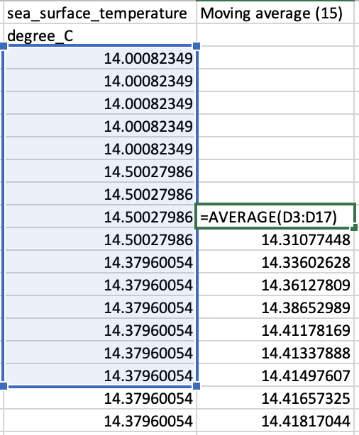
Figure 5: Calculating a moving average with a window size of 15
When calculating a moving average, a little data is lost from the start and the end of the original range. The effect of this smoothing operation is shown in Figure 6 where the blue curve represents the orginal data, and the orange curve is the moving average. The larger the window, the more the original curve is smoothed.

Figure 6: Moving average compared to the original data
 Moving average
 Smoothing in Arduino code